Zafir's Blog

Bridging Flow & Diffusion

Mar 22, 2026

Diffusion models are pretty cool, but the different perspectives (score matching, flow matching, etc.) always felt disconnected to me. I thought it would be cool to try and fix that, but my research got complicated really fast. If you want to dive in yourself, these links were helpful:

arXiv: 2303.08797
ICML 2025 Talk
arXiv: 2208.14699
Conditional Flow Matching Blog
arXiv: 2503.21756v1
MIT Lecture Notes (good intro)
Sander Dieleman’s blog (another good intro)

Here are some of the simpler ideas I found.

Generative models

The problem of generative modeling is the problem of transforming noise to data. That way, generation can be done by sampling noise, and simultaneously there is some notion of data likelihood and modeling the data distribution.

Input: Data $\mathcal{D} = \{X_i\}_{i=1}^{n}$ from an unknown distribution $P_{\mathrm{data}}$.

Goal: Learn a generator that can sample from $P_{\mathrm{data}}$ via

\[X = T_\theta(Z), \quad Z \sim P_{\mathrm{noise}}.\]

Process models

In the past, these $T_\theta$ models were “one-step” models (GANs, VAEs, etc.), but recently the strongest models are instead “process” models, where $T_\theta$ is iterative (flow, diffusion, GPT, etc.)¹. For example, generating an image via diffusion might take hundreds of passes through the model.

The learning process via expectation maximization (EM) has also changed. The canonical example from the past here is the VAE:

VAE optimization is centered around maximizing the log likelihood of generating the data (expectation maximization via the ELBO)

This is done by:

estimating the posterior distribution $Q_\phi(Z \mid X = x_i)$ given some data observation $x_i$ (E-step, aka the encoder)
learning $\theta$ from the imputed $z_i \sim Q_\phi(Z \mid X = x_i)$ (M-step, aka the decoder)
$Q_\phi$ and $P_\theta$ are iteratively updated to fit each other and maximize the ELBO.

\[Q_{\phi}\;\overset{\text{M step}}{\underset{\text{E step}}{\rightleftarrows}}\;P_{\theta}\]

The new approach only involves the M-step, with $Z$ instead drawn from some fixed, unparametrized, simple process $\mathbb{Q}$ (think the noising process used in DDPM).

\[\mathbb{Q}\;\overset{\text{M step}}{\rightarrow}\;P_{\theta}\]

Why do this?

With large neural networks, the model space is so rich that $P_\theta$ can invert any $\mathbb{Q}$ (“universal approximator”)
We can still find an MLE solution in this framework; it was never unique anyway
Simpler and more efficient training (one model instead of two, no “moving targets”)

Building process models

Let’s make this concrete. The $\mathbb{Q}$ process determines some latent distribution, and via the model, now dictating some process, we want to transform those points to draw from the data distribution. In other words: we need a process that transforms one distribution into another. Such a process is sometimes called a bridge (haha get the title?).

Since our objects of interest (images, for example) can be represented as vectors, it’s very natural to study this transformation in the language of ODEs and SDEs:

A trajectory is a map

\[X:[0,1]\to\mathbb{R}^d,\quad t\mapsto X_t.\]

A vector field defining an ODE is a map specifying a velocity in space

\[u:\mathbb{R}^d\times[0,1]\to\mathbb{R}^d,\quad (x,t)\mapsto u_t(x).\]

Then, a flow is the trajectory generated by this ODE:

\[\psi:\mathbb{R}^d\times[0,1]\to\mathbb{R}^d,\quad (x_0,t)\mapsto \psi_t(x_0),\] \[\frac{d}{dt}\psi_t(x_0)=u_t\big(\psi_t(x_0)\big),\quad \psi_0(x_0)=x_0.\]

Under mild assumptions, the flow exists and is unique. We usually can’t solve it exactly, so we simulate it numerically (e.g., Euler’s method). Indeed, ODE simulation is a well-studied topic and there are many powerful methods.

We can extend the ODE view to an SDE by adding Brownian noise (Wiener process $W_t$)². Since Brownian paths are not differentiable, we write the dynamics in differential form³:

\[dX_t = f_t(X_t)\,dt + \sigma_t\,dW_t,\quad X_0 = x_0.\]

where $\sigma_t$ is the diffusion coefficient which we can set. How do we simulate an SDE? Due to the properties of the Wiener process, we only need to modify Euler’s method slightly:

\[\begin{gathered} \operatorname{\text{Euler method}\ (ODE)}\\ x_{k+1} = x_k + h\,u_{t_k}(x_k),\quad t_k = kh. \end{gathered}\] \[\begin{gathered} \operatorname{\text{Euler-Maruyama method}\ (SDE)}\\ x_{k+1} = x_k + h\,f_{t_k}(x_k) + \sigma_{t_k}\sqrt{h}\,\varepsilon_k,\quad \varepsilon_k \sim \mathcal{N}(0, I). \end{gathered}\]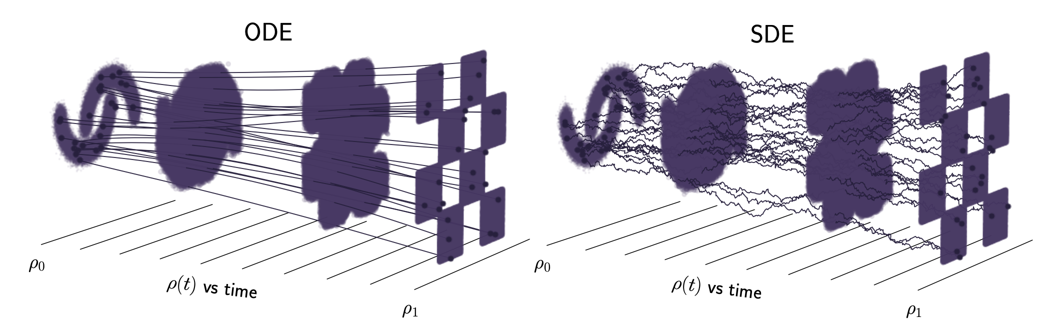

Lastly, having introduced stochasticity, the idea of a “probability path” is intuitive: if $X_0 \sim p_0$, the dynamics induce a distribution at each time $t$:

\[p_t := \text{distribution of } X_t \text{ at time } t,\quad t\in[0,1].\]

For a better treatment of all of this, see MIT Lecture Notes.

Learning flow models

Now, we understand our goal. We want to learn a velocity vector field $u_t^\theta(x_t)$ parameterized by a neural network that induces a probability path with the right endpoints:

\[p_0 = P_{\mathrm{noise}},\qquad p_1 = P_{\mathrm{data}}.\]

If we have this field, we can simulate the flow to sample from the data distribution. Under the SDE framework, this is called a diffusion model, but let’s start with the simpler, special case of $\sigma_t = 0$, a flow model. Conceptually, we want to match a target marginal velocity field $u^*_t(x_t)$ that dictates our desired probability flow, but it’s not immediately clear how to do this.

The simple process $\mathbb{Q}$ (E-step) we established earlier can help. For example, under the standard Gaussian noising process, we can write the probability path conditioned on a single data point $x$:

\[p_t(x_t \mid x) = \mathcal{N}(x_t; \alpha_t x, \beta_t^2 I_d)\]

$\alpha_t$ scales the data. As $t$ goes backward from $1$ to $0$, it scales the data point down to zero ($\alpha_1 = 1 \to \alpha_0 = 0$).
$\beta_t$ scales the noise. As $t$ goes backward from $1$ to $0$, it increases the variance until it reaches standard normal noise ($\beta_1 = 0 \to \beta_0 = 1$).

With this defined probability path, we can actually derive a completely tractable conditional velocity, $u_t^{\mathrm{cond}}(x_t \mid x)$:

\[u_t^{\mathrm{cond}}(x_t \mid x) = \left(\dot{\alpha}_t - \frac{\dot{\beta}_t}{\beta_t}\alpha_t\right)x + \frac{\dot{\beta}_t}{\beta_t}x_t\]

Derivation

A sample $x_t$ from the conditional distribution $p_t(x_t \mid x)$ can be written using the reparameterization trick with standard Gaussian noise $\epsilon \sim \mathcal{N}(0, I_d)$: $$ x_t = \alpha_t x + \beta_t \epsilon $$ To find the velocity, we take the time derivative of this path: $$ \dot{x}_t = \dot{\alpha}_t x + \dot{\beta}_t \epsilon $$ We are almost done, but the velocity should be a function of the position $x_t$, not some external variable $\epsilon$. We can solve our first equation for $\epsilon$: $$ \epsilon = \frac{x_t - \alpha_t x}{\beta_t} $$ Then, substituting $\epsilon$ back yields the conditional velocity: $$ \begin{aligned} u_t^{\mathrm{cond}}(x_t \mid x) &= \dot{\alpha}_t x + \dot{\beta}_t \left( \frac{x_t - \alpha_t x}{\beta_t} \right) \\ &= \left(\dot{\alpha}_t - \frac{\dot{\beta}_t}{\beta_t}\alpha_t\right)x + \frac{\dot{\beta}_t}{\beta_t}x_t \end{aligned} $$

which we can use for the marginal velocity:

\[u^*_t(x_t) = \int u_t^{\mathrm{cond}}(x_t \mid x)\,\frac{p_t(x_t \mid x)\,P_{\mathrm{data}}(x)}{p_t(x_t)}\,dx = \mathbb{E}_{x \mid x_t}[u_t^{\mathrm{cond}}(x_t \mid x)]\]

Then, our ideal objective would be to match this marginal velocity:

\[\mathcal{L}_{\mathrm{FM}}(\theta) = \mathbb{E}_{t, x_t}\big[\|u_t^\theta(x_t) - u^*_t(x_t)\|^2\big]\]

But again we get stuck because $u^*_t(x_t)$ includes an intractable integral.

The breakthrough of flow matching is noticing that we can sidestep this intractable integral. Instead of regressing against the marginal velocity, we regress directly against the tractable conditional velocity:

\[\mathcal{L}_{\mathrm{CFM}}(\theta) = \mathbb{E}_{t, x_t, x}\big[\|u_t^\theta(x_t) - u_t^{\mathrm{cond}}(x_t \mid x)\|^2\big]\]

We can show it is equivalent:

\[\mathcal{L}_{\mathrm{CFM}}(\theta) = \mathcal{L}_{\mathrm{FM}}(\theta) + C\]

Thus their gradients match, and we arrive at the same minimizer!

Proof

We expand the conditional loss function: $$ \begin{aligned} \mathcal{L}_{\mathrm{CFM}}(\theta) &= \mathbb{E}_{t, x_t, x}\big[\|u_t^\theta(x_t) - u_t^{\mathrm{cond}}(x_t \mid x)\|^2\big] \\ &= \mathbb{E}_{t, x_t, x}\big[\|u_t^\theta(x_t)\|^2 - 2\langle u_t^\theta(x_t), u_t^{\mathrm{cond}}(x_t \mid x)\rangle\big] + \underbrace{\mathbb{E}_{t, x_t, x}\big[\|u_t^{\mathrm{cond}}(x_t \mid x)\|^2\big]}_{:= C_1 \text{ (indep. of } \theta)} \end{aligned} $$ Next, we apply the law of iterated expectations ($\mathbb{E}_{t, x_t, x} = \mathbb{E}_{t, x_t}\mathbb{E}_{x \mid x_t}$). Since $u_t^\theta(x_t)$ is independent of $x$ given $x_t$, we can factor it out: $$ \begin{aligned} \mathcal{L}_{\mathrm{CFM}}(\theta) &= \mathbb{E}_{t, x_t}\left[ \|u_t^\theta(x_t)\|^2 - 2\big\langle u_t^\theta(x_t), \mathbb{E}_{x \mid x_t}\left[u_t^{\mathrm{cond}}(x_t \mid x)\right] \big\rangle \right] + C_1 \end{aligned} $$ By definition, the inner expectation $\mathbb{E}_{x \mid x_t}[u_t^{\mathrm{cond}}(x_t \mid x)]$ is exactly the marginal field $u^*_t(x_t)$. Substituting this back in: $$ \begin{aligned} \mathcal{L}_{\mathrm{CFM}}(\theta) &= \mathbb{E}_{t, x_t}\big[\|u_t^\theta(x_t)\|^2 - 2\langle u_t^\theta(x_t), u^*_t(x_t)\rangle\big] + C_1 \end{aligned} $$ Finally, we complete the square by adding and subtracting $\mathbb{E}_{t, x_t}[\|u^*_t(x_t)\|^2]$: $$ \begin{aligned} \mathcal{L}_{\mathrm{CFM}}(\theta) &= \mathbb{E}_{t, x_t}\big[\|u_t^\theta(x_t) - u^*_t(x_t)\|^2\big] - \underbrace{\mathbb{E}_{t, x_t}\big[\|u^*_t(x_t)\|^2\big]}_{:= C_2 \text{ (indep. of } \theta)} + C_1 \\ &= \mathcal{L}_{\mathrm{FM}}(\theta) + C \end{aligned} $$

Coming eventually: connecting to score matching and diffusion

Some include residual networks in this list, which I thought was interesting to think about. ↩
Why extend the ODE to an SDE? Actually, in some diffusion literature, the stochastic view came first; practically, the noise can improve robustness and often gives better results. ↩
$f_t$ is used, not the flow velocity $u_t$, because adding noise fundamentally alters the dynamics needed to maintain the same probability path, which we will unpack later. ↩