VAEs

Before variational autoencoders (VAEs) there were autoencoders. They attempt to learn the identity function by encoding into a lower dimensional latent then decoding back to the original input. With this “bottleneck,” we can get a compressed representation of the input.

VAEs are less straightforward; they map inputs to latent distributions and explicitly model the data distribution. Modeling the data distribution gives generative capability. For example, working with latent distributions rather than points prevents the model from becoming a “lookup table” as the in-betweens become meaningful and interesting.

Modeling the distribution

It is common to call the data input $x$ and the latent $z$. From before, we map inputs to a distribution, call it $p_\theta$, parameterized by $\theta$. Then under the Bayesian framework we can consider:

• The prior, $p_\theta(z)$ (the distribution of the latent space, before data)
• The likelihood, $p_\theta(x \mid z)$ (given a latent $z$, what is the distribution of data $x$ it decodes to)
• The posterior, $p_\theta(z \mid x)$ (given a data $x$, what is the distribution of latents $z$ it encodes to)
• The evidence, $p_\theta(x) = \int p_\theta(x \mid z)p_\theta(z)dz$ (the marginal distribution of the data under the model)

The evidence hints at our generative process. We will sample a $z_i \sim p_\theta(z)$, then sample $x_i \sim p_\theta(x \mid z_i)$.

For choosing $\theta$, we want to maximize the probability of generating real data (the maximum likelihood estimate), i.e. we want:

Unfortunately this is intractable, as we can’t integrate over all dimensions of the latent space.

This is solved using a technique called variational inference (VI). It is suited for the problem of approximating the posterior, which is $p(z \mid x)$ in our case. Approximating $p(z \mid x)$ is of interest because from Bayes’ rule, for any given latent z:

It’s now possible because it’s a bit circular—normally we use $p_\theta(z \mid x) = \frac{p_\theta(x, z)}{p_\theta(x)}$.

With VI, we select a family of probability distributions $\mathcal{Q}$, then find the “closest” $q(z \mid x) \in \mathcal{Q}$ to $p(z \mid x)$ (using gradient descent). It’s in our interest to select a “nice” $\mathcal{Q}$—then the $q_\phi(z \mid x)$, parameterized by $\phi$, that we get back is easy to evaluate and close enough so we can use it instead of $p(z \mid x)$.

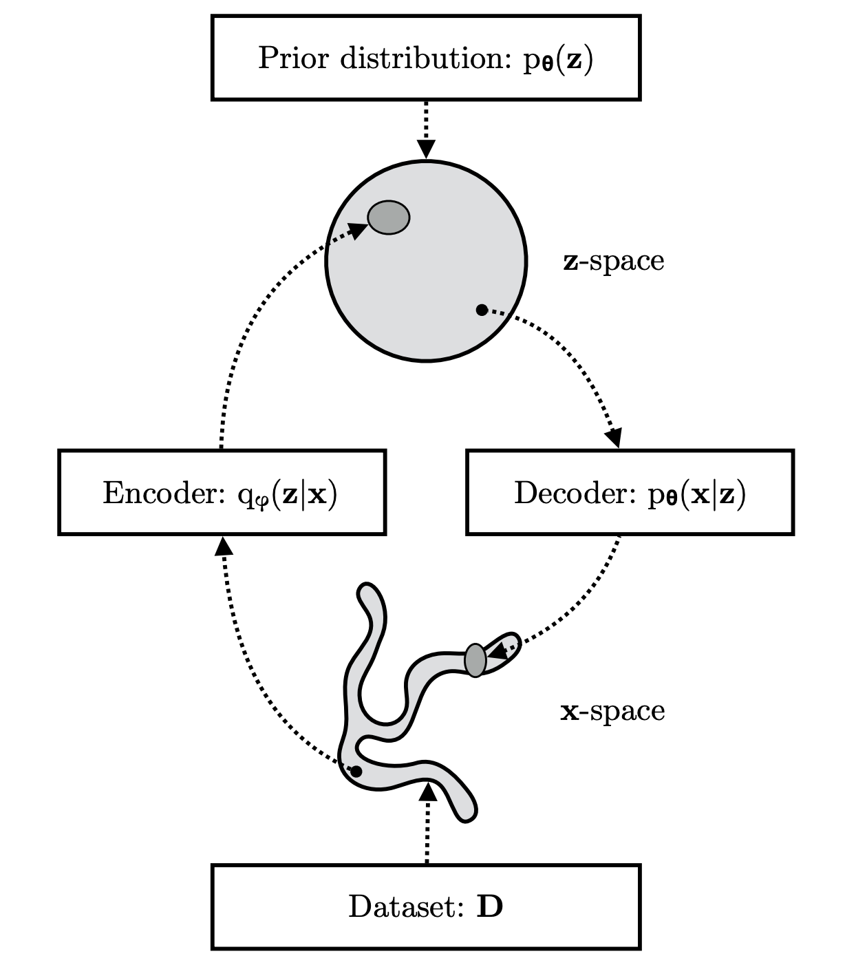
In the end, our autoencoder consists of these two:

• $p_\theta(x \mid z)$, the generative model, also called a probabilistic decoder.
• $q_\phi(z \mid x)$, the posterior approximation, called the probabilistic encoder.

They are useful for $p_\theta(x_i)$, as given in $\eqref{eq:bayes}$. What about $p_\theta(z)$? Since we ultimately want to generate new images, i.e. sample $z_i \sim p_\theta(z)$, we will make it simple, like a Gaussian.

ELBO

Ideally, the objective function for our autoencoder will allow us to jointly optimize $\theta, \phi$. A good choice is the evidence lower bound (ELBO), commonly used with VI. As indicated by the name, it’s often motivated by considering the evidence $p_\theta(x_i)$ (which we are definitely interested in):

The second term is the Kullback-Leibler (KL) divergence between $q_\phi(z \mid x_i)$ and $p_\theta(z \mid x_i)$, which quantifies how different the distributions are. KL divergence is always non-negative:

where at $\text{(a)}$ we use Jensen’s inequality, $\log$ being concave. So, rearranging $\eqref{eq:elbo}$:

Notice that if we maximize the LHS, we both maximize the log probability of generating real data ($\log p_\theta(x_i)$) AND minimize the difference between the real and approximate posterior—exactly our goal when optimizing $\theta, \phi$. In addition to that, we directly improve a lower bound of the evidence $p_\theta(x_i)$, giving the ELBO its name.

Reparameterization trick

With this ELBO objective that we have defined, we would like to improve our autoencoder’s $\theta, \phi$ using stochastic gradient descent (using a sample/subset of the dataset to estimate the true gradient). Then, we want the gradient w.r.t. our parameters. For $\theta$ it’s not so bad:

where we sample $z_j \sim q_\phi(z \mid x_i)$, and the last line is an unbiased estimator for the gradient. For $\phi$, it’s more difficult because in general:

Intuitively, we cannot move the gradient inside the expectation because it would ignore how changing $\phi$ might also shift the “cloud” of samples (and thus the expectation).

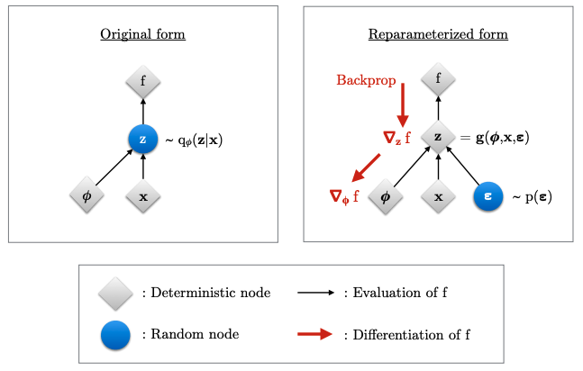
This is solved through a change of variables called the “reparameterization trick,” where we represent the random variable $z \sim q_\phi(z \mid x)$ as a deterministic, differentiable transformation of $\epsilon$, some independent auxiliary random variable:

Then, expectations can be rewritten in terms of $\epsilon$:

where $z = g(\phi, x, \epsilon)$ with $\epsilon \sim p(\epsilon)$.

Theory will only take you so far

We’ve shown we can compute the gradients, but that’s not enough to code it in PyTorch. Let’s do the final steps:

Let’s motivate the first term being the reconstruction error. First, what is $p_\theta(x_i \mid z)$? In practice, our model won’t actually output a distribution (it’s not necessary). It will really just map some latent $z_j$ deterministically to a reconstructed data input $f_\theta(z_j)$.

We need a distribution for our gradient though, so to make minimal assumptions we can assume there is some noise around $f_\theta(z_j)$ which is the mean—essentially, a Gaussian (the maximum entropy distribution in this case). With this “wrapper” we can treat the gap between our output and the actual data as a likelihood:

where C is irrelevant to the gradient and our imaginary noise level only functions as a scaling factor.

Next is the regularization. Recall the KL divergence quantifies how different the distributions are. Then, optimizing $\phi$ involves bringing an input’s latent distribution closer to the prior distribution. This regularizes the latent space by preventing the encoder from collapsing into a lookup table, forcing it to learn a continuous, overlapping representation.

But how do we compute it? First, we need to define a few things. For $p_\theta(z)$, as hinted at from before, typically $\mathcal{N}(0,I)$ is used (simple to sample, maximum entropy). Similarly, $\epsilon \sim \mathcal{N}(0,I)$, and via transformation we make $q_\phi(z \mid x_i)$ a multivariate Gaussian with a diagonal covariance matrix (tractable but still expressive[^1]):

where $\odot$ is an element-wise product.

Then, we want the KL divergence between these two Gaussians. Because $q_\phi$ has a diagonal covariance matrix, its dimensions are independent, allowing us to factor the joint probability density into a product of marginal densities ($p(a,b) = p(a)p(b)$). Since KL divergence acts on the log of these densities, and by linearity of expectation, the total divergence becomes a sum of independent, one-dimensional divergences. Then, the problem reduces to $D_{KL}(q \Vert p) := \mathbb{E}_{z \sim q}[\log q(z) - \log p(z)]$ where $q(z)=\mathcal{N}(\mu,\sigma^2)$ and $p(z)=\mathcal{N}(0,1)$ for each dimension independently:

Finally, we arrive at the “canonical” VAE loss, something we can actually code in PyTorch:

def vae_loss(x, x_hat, mu, log_var):
    recon_loss = (x - x_hat).pow(2).flatten(1).sum(1).mean()

    kl_loss = 0.5 *
    (-log_var - 1 + mu.pow(2) + log_var.exp()).sum(1).mean()

    return recon_loss + kl_loss