Notes

Here are the unedited notes that I made during the project. There are a lot of helpful links if you are studying on your own, as well as some content I haven’t gotten around to adding to the site yet, such as RNNs, so feel free to look around!

Sorry about some of the really large images—I exported these notes directly from notion.

Datacamp
- https://app.datacamp.com/learn/courses/introduction-to-deep-learning-in-python
- https://app.datacamp.com/learn/courses/supervised-learning-with-scikit-learn
Google’s machine learning course
TensorFlow’s resources
- https://www.tensorflow.org/resources/learn-ml
- https://www.tensorflow.org/tutorials/images/classification
Kaggle
- https://www.kaggle.com/datasets?tags=14102-Image+Data
Stanford Convolutional Neural Network class
- https://cs231n.github.io/

Goals for the project

Image Classifier (mask clasifier)
Neural net from scratch?

General machine learning workflow

Examine and understand the data
Build an input pipeline of the data
Build our model
Train our model
Test our model
Improve the model and repeat the process!

Udacity, Intro to TensorFlow for Deep Learning

Link to course

Deep Learning: a subfield of machine learning that uses multi-layered neural networks, often used interchangeably with “deep learning”
- many subfields, branches, etc
  - Supervised vs unsupervised learning
Colab is similar to jupyter notebook (which I have experience with)
- Numpy!

Creating the first model

create a model

  import tensorflow as tf
  import numpy as np
    
  model = tf.keras.Sequential([
    tf.keras.layers.Dense(units=1, input_shape=[1])
  ])

compile the model

  model.compile(loss='mean_squared_error',
                optimizer=tf.keras.optimizers.Adam(0.1))

train the model!

  history = model.fit(celsius_q, fahrenheit_a, epochs=500, verbose=False)

Gradient descent simply is nudging the parameters in the correct direction until they reach the best values, where any more nudges would

Stochastic Gradient Descent (SGD)
- Gradient calculated for each example rather than every “step”
- Batch size of 1, in relation to BGD
Batch Gradient Descent (BGD)
- Model updated after calculating gradient for every example
- Mini-batch: variation, where only part of the examples is evaluated rather than all of them
  - Reduces noise of SGD but more efficient than BGD
Dense layer: every node is connected to every node in the previous layer
- each node has a weight for each node in the previous node (slope), and one bias (y-intercept)

Image Classification with NMIST

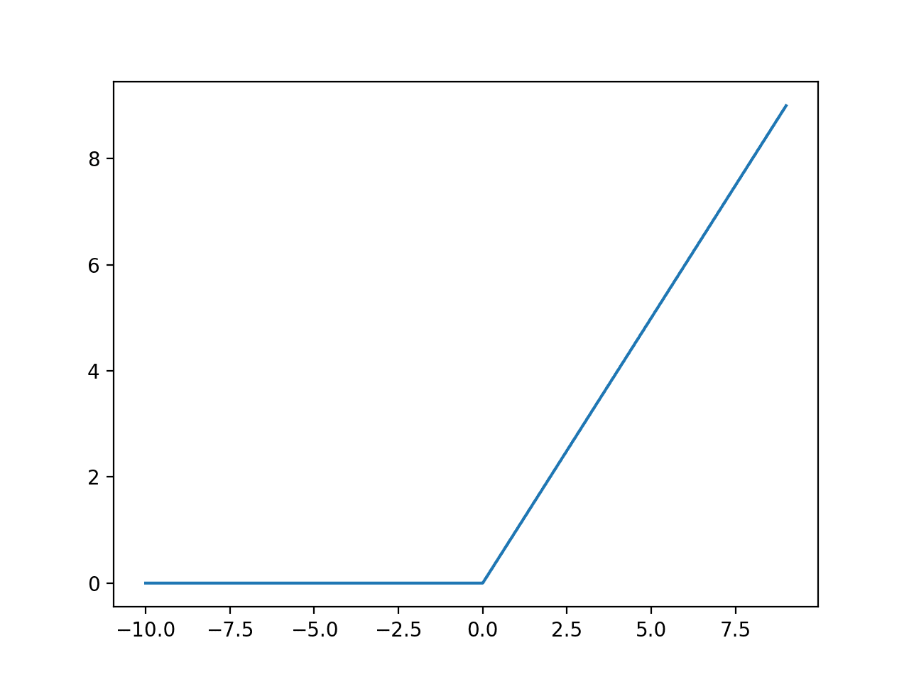
ReLU: activation unit, “Rectified Linear Unit”
- adds functionality of adapted to non-linear functions
- 0 and negative values map to 0, otherwise map to x (input)
- applied to hidden layer (between input and output)
- able to account for interaction effects (where one variable influences if one should or should not be considered

softmax: provides probabilities for each output, used for classification
overfitting: sometimes the model can memorize the training data, but preform badly on generalized input. this is undesirable, therefore we need a validation/testing data to evaluate the model
- result of bias-variance trade off: variance can be adjusted by shifting bias in accordance with training data, reducing variance
- high bias error: erroneous assumptions → poor generalization, under-fitting
- variance error: high variance in training data → model random noise in training data (overfitting)
- more parameters → more random solution
- solutions:
  - cross-validation: periodically verify with testing data, stop when testing data accuracy goes down
  - constrain bias closer to zero
a lot of work is with data, 90% is cleaning up

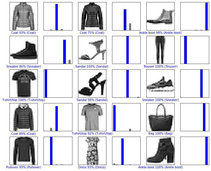
Even after messing around, the highest accuracy I could get was 89%, but thats good considering humans get an accuracy of 93%

Convolutional Neural Networks

proven to be better for image classification
uses two new concepts: convolutions and max-pooling
a convolutional layer uses another layer of numbers, known as the kernel, and uses it to create a convoluted layer
use zero padding for edge
max pooling: process of reducing image size by summarizing input
- uses grid size and stride

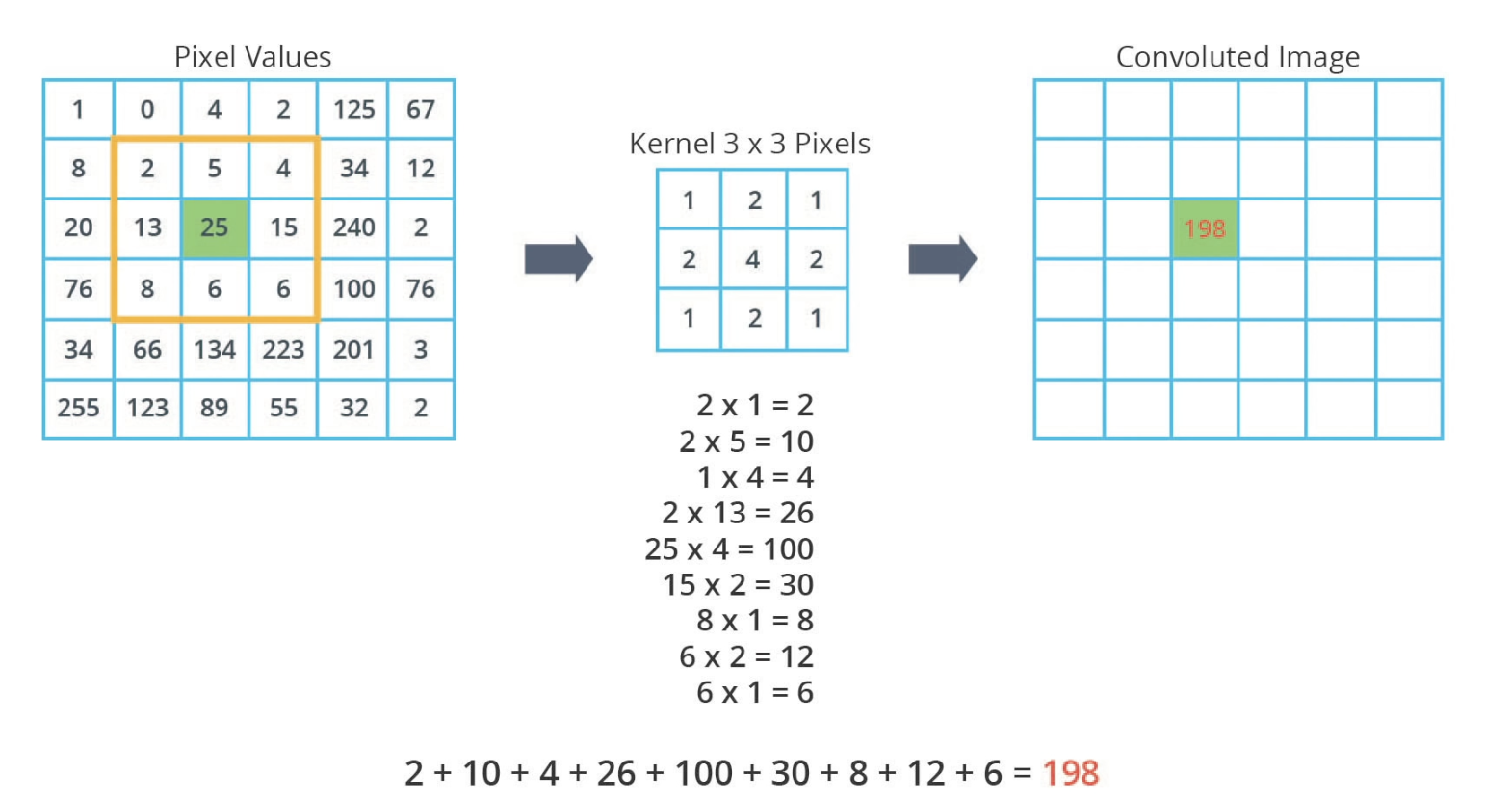
Kernel and convolutions

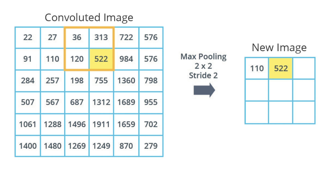
Max pooling

model = tf.keras.Sequential([
    tf.keras.layers.Conv2D(32, (3,3), padding='same', activation=tf.nn.relu,
                           input_shape=(28, 28, 1)),
    tf.keras.layers.MaxPooling2D((2, 2), strides=2),
    tf.keras.layers.Conv2D(64, (3,3), padding='same', activation=tf.nn.relu),
    tf.keras.layers.MaxPooling2D((2, 2), strides=2),
    tf.keras.layers.Flatten(),
    tf.keras.layers.Dense(128, activation=tf.nn.relu),
    tf.keras.layers.Dense(10, activation=tf.nn.softmax)
])

CNN with color images

dealing with images of different sizes → resize to set amt of pixels → all result in flattened images with same size
dealing with color images: 3 dimensional array, width, height, color channels
- rather than (28,28,1) input, use (150,150,3)
- use 3D filter! use each layer separately, and on the same pixel at the same time
- add colors and add bias value

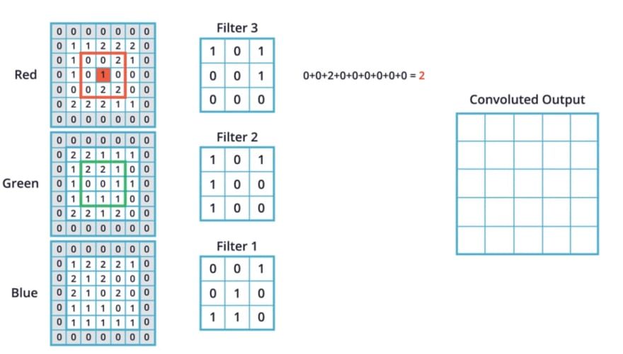
use multiple filters for multiple convoluted images, create 3D array again
max pooling is the same for each convoluted image
it’s also possible to use Dense layer with 1 output and a sigmoid activation function (for binary classification)
- loss parameter will have to train
validation set during training
- simply check how the model is doing on the validation set, do not use it to tune weights and biases
- gives idea of how generalizes
- compare between models
- STILL need a test set to see how model generalizes, since the model is still biased towards the validation set
dropout
- randomly turn off some neurons during training, forcing other neurons to “do more work”
- good when some neurons are doing a “lot of the work”
- network becomes more resistant and better at not overfitting, since not every neurons is being used
early stopping
- track loss on validation and stop training before it begins to increase after a certain point

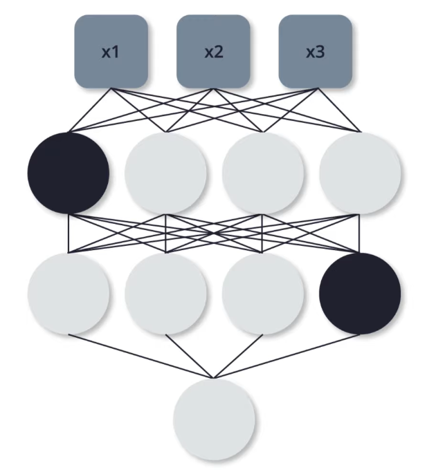
The black neurons are said to be “dropped out”

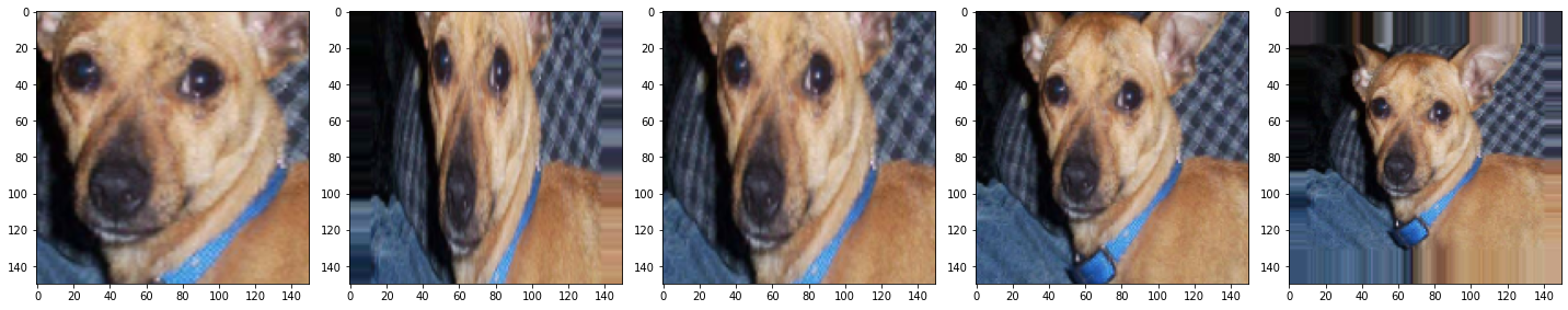
data augmentation
- overfitting happens when we have small # of training examples
- this approach generates more training data from existing samples through random transformations
- accuracy goes up and less overfitting!!

image_gen_train = ImageDataGenerator(
      rescale=1./255,
      rotation_range=40, # rotate up to 40 degrees
      width_shift_range=0.2, # shift keeping width
      height_shift_range=0.2, # shift keeping height
      shear_range=0.2, # shift image like parallelogram
      zoom_range=0.2, # zoom in our out
      horizontal_flip=True, # randomly apply horizontal flips
      fill_mode='nearest') # fill blank pixels with nearest non-blank

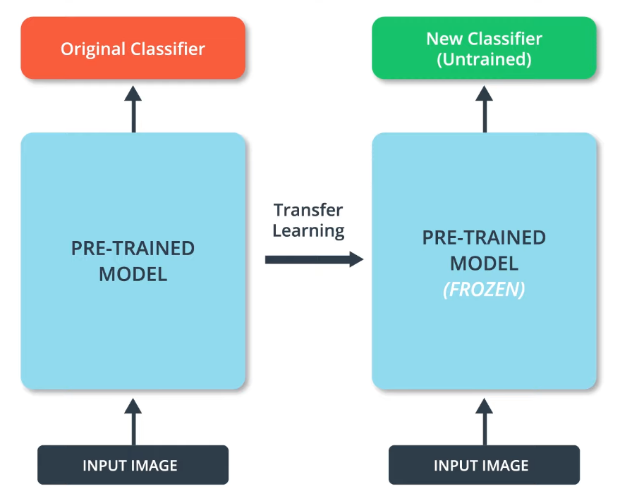
Transfer Learning

transfer models to another purposes
- similar to school (first 18 years)
take the pre-trained model, freeze it, and attach a new classifier at the end to adapt to the new task
use MobileNet (very efficient, little memory, able to run on mobile devices)
https://www.tensorflow.org/hub: Hub of trained machine learning models
faster training, needing less data, and better performance

CLASSIFIER_URL ="[insert url from tf]"
IMAGE_RES = 224

model = tf.keras.Sequential([
    hub.KerasLayer(CLASSIFIER_URL, input_shape=(IMAGE_RES, IMAGE_RES, 3))
])

a feature extractor does everything but classify the images
- in essence, it is the entire model without the last layer, thus it has extracted the features of the image

Time Series Forecasting

a trend in data is an overall change, usually just increase or decrease
seasonality in data is a recurring pattern of changes, usually related to the season or day of the week

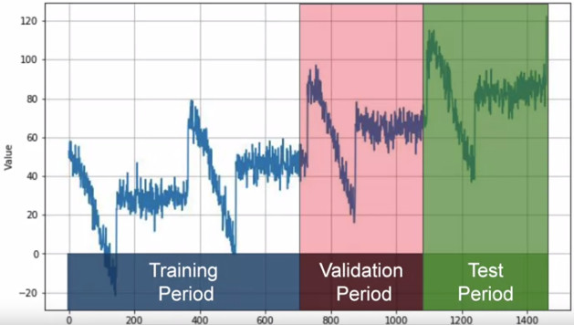
How do we partition data, now that, instead of images, we have linear data?

Fixed partitioning
- Simply breaking the data into a training, validation and test period, similar to image classification
- In practice, before deployment the model is trained on the validation and test data as well, since those periods are most recent and therefore most significant as data

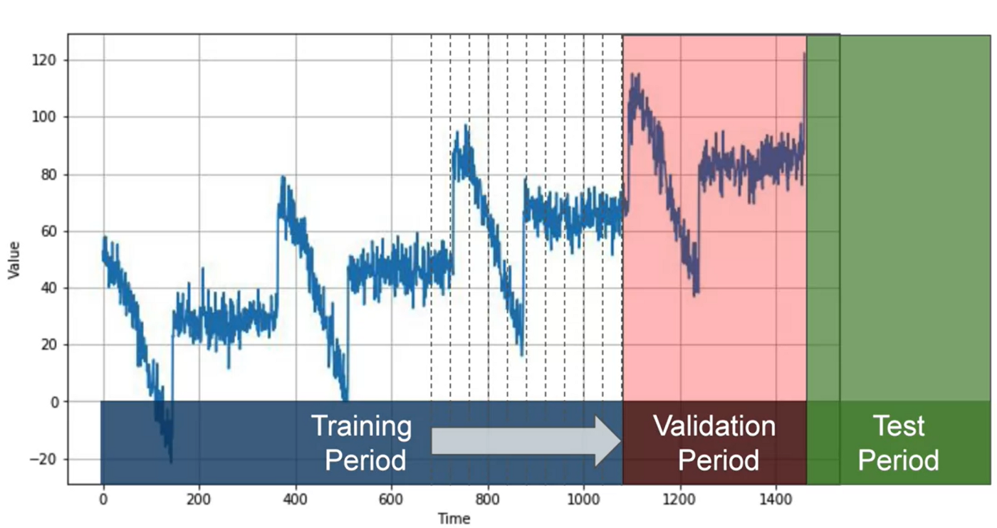
Roll-forward partitioning
- Train through training data in small partitions, where the model successively predicts what happens in each smaller partition and learns (like it is “rolling forward” through the training data)
- Slower than fixed partitioning

error = series-forecast

MSE: mean-squared error, penalizes high errors more
MAE: mean-abs error
Differencing
- Convert the data from series(t) to series(t)-series(t-365), eliminating seasonality
- Combining with rolling average, we can eliminate noise and get a MAE a bit better than the naive forecast
  - We can use centered windows rather than trailing windows, since we have access to the data of the entire last year
  - This solution is often not too far from optimal, while simple

dataset = tf.data.Dataset.range(10)
dataset = dataset.window(5, shift=1, drop_remainder=True)
dataset = dataset.flat_map(lambda window: window.batch(5))
dataset = dataset.map(lambda window: (window[:-1], window[-1:]))
dataset = dataset.shuffle(buffer_size=10)
dataset = dataset.batch(2).prefetch(1)
for x, y in dataset:
    print("x =", x.numpy())
    print("y =", y.numpy())

Recurrent Neural Networks (RNN)

contains recurrent layers, that can sequentially process a sequence of inputs
- used for time series, sentences

Recurrent Layer

composed of single memory cell, which is repeatedly used
each memory cell is a neural network, like a Dense layer or LSTM
each memory cell has a normal output, as well as a state or context vector
- this state vector is fed as an additional input to the next memory cell
input shape is 3-dimensional:
- batch size e.g. 4 windows
- num time steps e.g. 30 steps per window
- num dimensions e.g. 1 (univariate data)

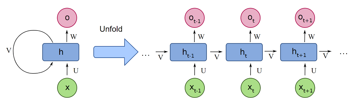
Here the layer is shown unfolded, with the state vector given as input to a repeated memory cell

Output shape depends on the number of neurons, or units, inside the memory cell.

Input a (4,1,30) shape tensor → Let’s say the memory cell has 3 neurons → (4,3,30) shape output, also 3-dimensional like input
In a simple RNN, there is only one neuron (a Dense neuron) and the state matrix/vector is just a copy of the output matrix

By default in Keras the RNN is “sequence-to-vector,” meaning instead of outputting a series of vectors there is just one, the last vector

This can be changed by the following code

model = keras.models.Sequential([
	keras.layers.SimpleRNN(100, return_sequences=True,input_shape=[None,1]),
	keras.layers.SimpleRNN(100),
	keras.layers.Dense(1)
])

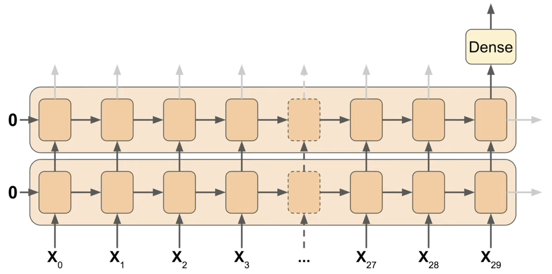
Model created by preceding code

return_sequences is set to True, meaning the first layer outputs everything
The input shape is odd. This is because Keras knows the first dimension is batch size, which it can adapt to any size. However the second dimension, the # of time steps, is set to None. This means that the RNN will handle sequences of any length, which is possible due to the repeatability of the memory cell. The final dimension is 1, as the data is univariate

Why no activation function?

By default it is set the the hyperbolic tangent function
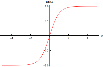
RNNs tend to have unstable gradients. Using a function like ReLu means the limit is unbounded (”non saturating”)

RNNs are tricky to train. Learning rate is very important and its effects are amplified, and the loss function will sometimes change randomly (could impede early stopping, set patience high and save checkpoints)

You are essentially training many neural networks, one per time step. Back-propagation, or in this case actually back-propagation Through Time (BPTT), goes through many nodes and very deep
- Gradients can vanish or explode going through many time steps
- Can be slow to predict long-term patterns
This can be sped up using a sequence-to-sequence approach instead of sequence-to-vector

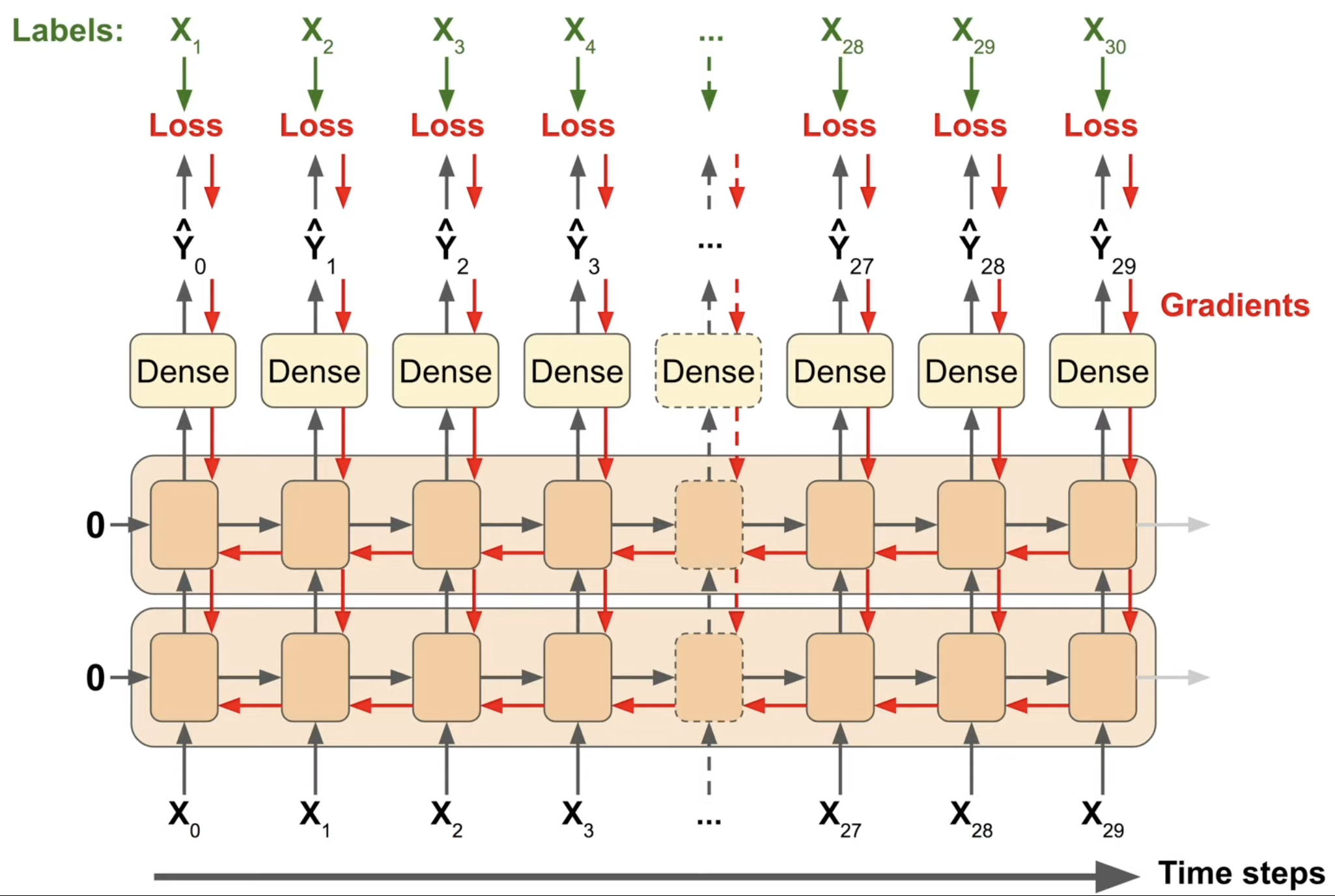
Each output is compared with the next input. This provides much more gradients for training, and if any one output had a high loss it would propagate more directly to the weights at that time step, speeding up training
- However this is still only used for training, in the end we only care about the last prediction
- In code, essentially each window is expanded by one and the last element is changed to the label
Never guaranteed good results. Sometimes it might just be better to use a moving average

Stateful RNN

A different approach, training RNNs completely differently. Until now we have used windows shuffled (anywhere in time range) with a state vector of 0, or stateless. In other words the model is forced to forget the context states from batch to batch. They are simple to use but cannot learn patterns longer than the window length.

We originally used stateless architecture was because we assumed the data was independent and identically distributed (IID). However, in temporal data, this is inherently not true, thus we might want to not reset the state matrix → stateful architecture

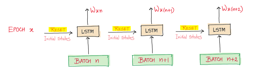
Stateless architecture

Stateful architecture (images taken from https://towardsai.net/p/l/stateless-vs-stateful-lstms)

Downsides are that data must be prepared differently, training can be slower, and adjacent time windows are very correlated so back-propagation might not work well
All of these make stateful RNNs much less used than stateless RNNs

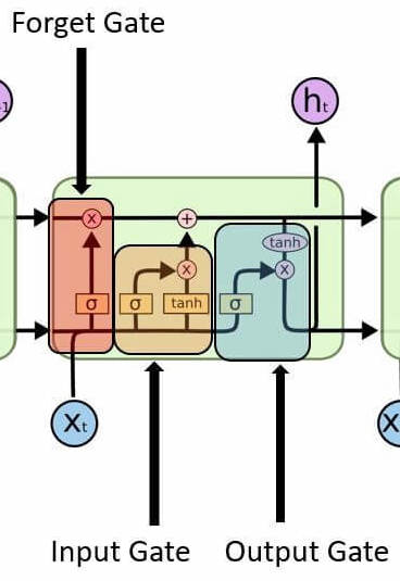
LSTM Cell (Long Short-Term Memory Cell)

Given a “longer” short-term memory, hence the name, and can detect patterns more than 100 time steps long

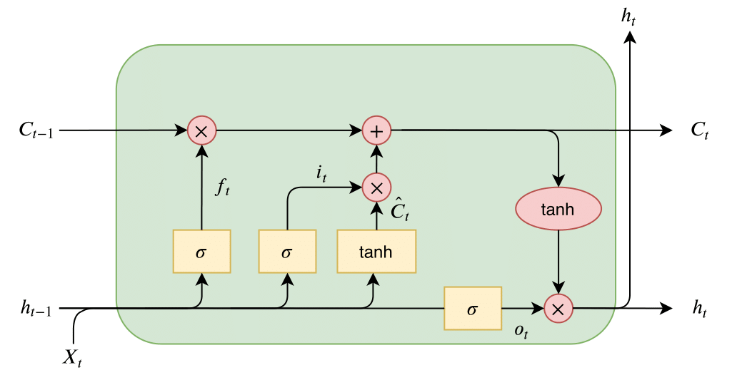
Note the yellow cells are preceded by Dense cells

Part of the cell is just a simple RNN cell: tanh, with inputs X_t and h_t-1
There is an added long-term state vector, represented as C_t; It goes through the cell with only two simple operations
- This helps gradients flow nicely through the vector, without exploding or vanishing
- Key idea of LSTM
Forget gate: a sigmoid function (0-1) is multiplied with the long-term state, causing it to be either erased (forgotten) or unchanged
- The model can learn when to erase part of the long-term memory, such as at the top of a sharp increase
Input gate: a sigmoid function is combined with tanh to create a gate that controls when something should be remembered, or added to LTM
Output gate: a sigmoid function combined with tanh from the LTM, learning which part of the LTM state should be output at each step
Can be used bidirectionally

GRUs (Gated Recurrent Unit) are quite similar to LSTM cells, with a reset and update gate, however it has less gates in total, often making it faster

Return of CNNs

Using a 1D-convolutional layer you can similarly include context. Analogous to using CNNs for 2D images but in 1D
Stacking multiple CNNs can address limitations, such as the window or kernel size
Padding: adding zeroes before or after, so that window sizes can be constant for all outputs - before is preferred (causal padding)
Strides: can shorten output and reduce computations
Kernels: change dimensionality of output, too many will overfit and two little won’t learn at all; ~32 normally

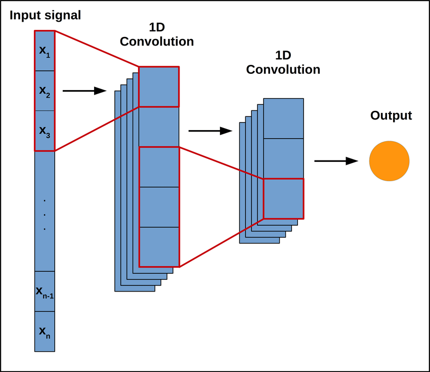
It’s possible to sidestep using RNNs completely, and it’s pretty popular for sequence processing. For example here is the WaveNet architecture

“Lower” layers learn short-term patterns while “higher” layers learn long-term patterns
2nd layer uses dilation of 2, 3rd uses 4, Nth uses 2^(N-1)
- dilation is like a stride, but in the input layer; dilation of 4 means 1 of every 4 inputs is taken
- each layer doubles the “receptive field”

Natural Language Processing (NLP)

NLP has many areas, such as sentiment analysis, dictation, translation, etc

Early uses were for translation, and did not use machine learning techniques

A tokenizer converts a # of the most common words in the dataset into numbers; The number of tokenized words is like the vocabulary size
- You can specify an OOV or out-of-vocabulary token for words that are not in this token set
- Now trained on very large text corpuses to avoid too many OOV words
  - https://github.com/niderhoff/nlp-datasets
  - https://datasetsearch.research.google.com/
However we need to preserve the order of words too, this is done with another text_to_sequences function

tokenizer = Tokenizer(num_words=20, oov_token=’OOV’) # creates token for 20 most common words
tokenizer.fit_on_texts(sentences) # applies tokenizer to input
tokenizer.texts_to_sequences(sentences) # creates tokenized sequence
print(tokenizer.word_index) # prints dictionary of word to token

We also need to pad sequences to make all sentences the same length; This is done with the pad_sequences function
Embedding are clusters of vectors, or words, in a multi-dimensional space
- It’s difficult for humans to imagine these dimensions so we have http://projector.tensorflow.org/
- These dimensions are determined through a variety of techniques, such as PCA (Principal Component Analysis), and T-SNE
  - These components, or dimensions, usually aren’t understandable by humans as they are made by machines

How a human might distribute features, or components, for a dataset (https://towardsdatascience.com/why-do-we-use-embeddings-in-nlp-2f20e1b632d2)

Very useful not only for saving memory but also for generalization, because, just like humans do, the model can understand new words from what they are related to, or its “neighbors”

model = tf.keras.Sequential([
    tf.keras.layers.Embedding(vocab_size, embedding_dim, input_length=max_length),
    tf.keras.layers.Flatten(),
    tf.keras.layers.Dense(6, activation='relu'),
    tf.keras.layers.Dense(1)
])
model.compile(loss=tf.keras.losses.BinaryCrossentropy(from_logits=True),optimizer='adam',metrics=['accuracy'])
model.summary()

model.fit(padded, training_labels_final, epochs=num_epochs, validation_data=(testing_padded, testing_labels_final))

How can we improve the model?

Increase vocabulary size (through the corpus); does not guarantee improvement, but will decrease the # of OOV words
More or fewer embedding dimensions
Flatten vs. Global Average Pooling (latter is often better)
Use subwords; let the model learn subwords instead of whole words → generalize better
- There are whole subword datasets or you can convert a corpus instead subword sets (breaks words into all subsets)

Text Generation

How do we generate text?

Simply train the model to predict the next word, then let it continue on
This can be done using the same model architecture and changing the output to a one-hot categorical class output, each class being a word
- There is more obvious changes to the data; Input data takes chunks of sequences, with the last word being its label

N-grams

The simplest text generation model would be one that assigns probabilities of a word given a certain history

https://towardsdatascience.com/introduction-to-language-models-n-gram-e323081503d9

One way to estimate this probability could be checking the corpus for how many times the history was followed by the possible new word. However this is slow, especially with large corpus sizes

An alternative is the Bigram model, which approximates the probability of a word using only the previous word
- Operates on the Markov assumption, which is, in this case, that the probability of the word depends only on the previous word
- This can be expanded to the trigram model → expanded to N-gram model

Downsides:

Very dependent on training corpus - sparse data, limited vocabulary
It’s repeating text!!!! What do we do!?!?!

Optimizations:

More data - consider memory and output size constraints
Keep tuning the model - layer sizes, embedding dimensions, hyperparameters
Use np.random.choice for more variance in outputs
Transformers 😈

Generative Adversarial Networks (GANs)

https://developers.google.com/machine-learning/gan

GANs are composed of two parts:

Generator: produces the target output
Discriminator: learns to differentiate real output from that of the generator

Both of these parts learn to get really good at their jobs, thus the generator produces (hopefully) realistic outputs. However, the generator has a harder problem to solve

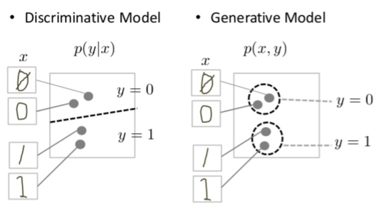
The discriminator need only find one small difference, while the generator must account for all of them. Thus, the generator has a harder job overall

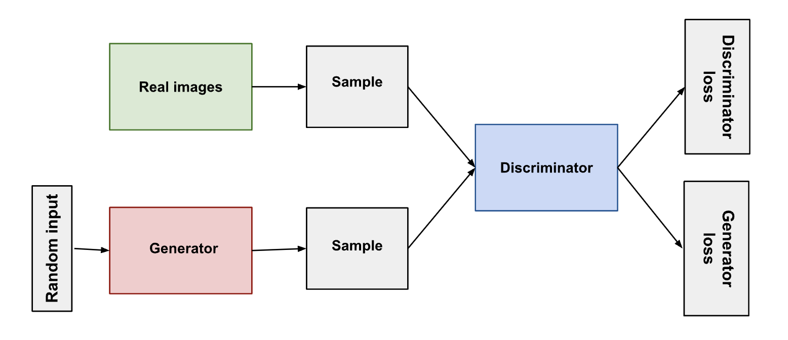
Model of system

The generator’s output is directly connected to the discriminators input, thus backpropagation can reach and update the generator’s weights
When the discriminator is being trained, the generator stays constant, and likewise vice versa. Otherwise, its like trying to hit a moving target. Thus after backpropagation for the generator, only the generator’s weights are updated.
The generator takes in random input, and changes it into its output. Through the random noise the generator can produce a wide variety of data.
The procedure alternates: first the discriminator trains for some # of epochs, then the generator
For a GAN, convergence (the desired state) is often fleeting. As the generator becomes better, the discriminator’s output become more and more meaningless. If the generator continues training past the point where the discriminator is essentially flipping a coin, it can start to produce junk

GANs often use a type of loss called Wassertein loss (default for TF-GAN, also called Earth mover’s distance). It involves a modification of the GAN scheme, called “WGAN,” where the discriminator does not actually classify but instead make its output larger for real data than fake data. Thus its called a “critic” instead of a discriminator

In this scheme, the discriminator attempts to maximize D(x) - D(G(z)) while the generator attempts to maximize G(z), D(x) being the critic’s output for real images and G(z) being the generator’s output given noise z

Problems:

If discriminator becomes too good, D(G(z)) = 0, then the generator has no gradient to train on aka the vanishing gradient problem
The generator is actively trying to create the output that the discriminator is most fooled by. If it accomplishes this, it might fixate on it while the discriminator is trapped at a local minimum. This is called mode collapse

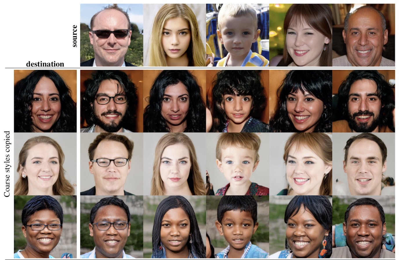
There are a wide variety of GANs. Shown here is StyleGAN which has multiple layers that progressively add details. These are called progressive GANs

Gradient-Based Learning

Using truth data to iteratively improve the performance of a model

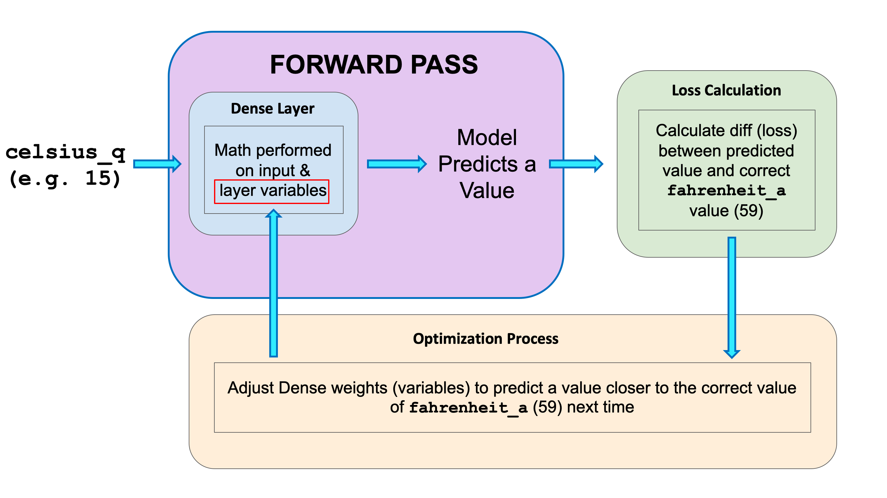
A forward pass is a mathematical mapping where parameters are applied to data to make its output. These parameters are refined so, for example, pictures of dogs are more consistently mapped to the “dog-like” classification, thus the machine “learns.”

loss (objective) function: mathematical function that provides a measure of how good a model is doing; the model is trained to reduce the output of the loss function
- takes as input the model (its parameters), the training data, and the truth data
- a gradient descent is consulted to gradually improve the parameters and reduce loss

If our model, L, has a single parameter, A, then we are trying to minimize a graph that is L(A)

We can compute the derivative of L(A), L’(A) with respect to A. This will tell us how changing A will change L(A). Let’s say L’(A) > 0. Since we are trying to minimize L(A), we will decrease A, since increasing it would also increase L(A) as L’(A) > 0. Formally, we iteratively update A via the following calculation, 𝛿 being the step-size

\[A_{new} = A_{old}-\delta \frac{dL}{dA}\ \bigg|_{A=A_{old}}\]

However, this is just a 2d function and valley. L can easily have millions of parameters and a “n+1” dimensional valley. The gradient is a vector that stores each of the derivatives, with respect to each of the parameter

When there is multiple variables, it is not as simple as “what is the slope,” because you must specify direction. Partial derivatives of a function, denoted as $\frac{\partial f}{\partial x}$, find the derivative with respect to one variable, holding the other variables constant

We can then find the derivative in any intermediate direction by using vectors. The gradient of $f(x,y)$ is the vector containing all the partial derivatives of f:

\[\nabla f(x,y)=[\frac{\partial f(x,y)}{\partial x},\frac{\partial f(x,y)}{\partial y}]\]

We can take the dot product of this gradient with a unit-vector in our direction of interest. For example the unit-vector pointing 45 degrees between +x and +y would be $\hat{u}=[\frac{1}{\sqrt{2}},\frac{1}{\sqrt{2}}]$. With the example of $f(x,y)=2x^2+xy$ we get

\[\nabla_{\hat{u}}f(x,y)=[\frac{1}{\sqrt{2}},\frac{1}{\sqrt{2}}]\cdot[4x+y,y]=\frac{4x+y}{\sqrt{2}}+\frac{x}{\sqrt{2}}=\frac{5x+y}{\sqrt{2}}\]

This generalizes: the dot product of a unit-vector with a gradient returns the derivative of f in the direction of the unit-vector. Additionally, $\nabla f$ points in the direction of steepest ascent (e.g. $[0,6,3]$), thus $-\nabla f$ points in the direction of steepest descent; This is exactly the direction we want to go to minimize f. Problems:

Unclear step-size (aka learning rate): if our step-size is too big, we might end up climbing instead of going down
- Important hyperparameter that one must use trial and error to improve
This method can find a local minimum, but that is not always the absolute minimum
The loss function must be differentiable, however this can pose a problem if trying to punish certain things e.g. failing twice in a row specifically

Neural Net from Scratch

Let’s make a neural net from scratch! I will be using this dataset: https://www.kaggle.com/datasets/uciml/iris?datasetId=19&searchQuery=scratch. Here are other helpful notebooks and resources:

I’m having trouble reconciling what I learned in Gradient Based Learning with the idea of the classic fully connected neural network

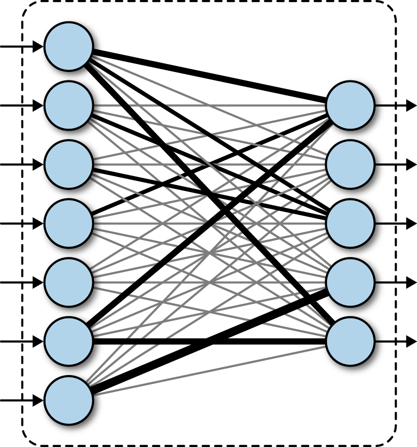
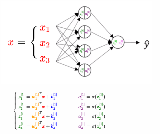
A fully connected layer in a deep network. A deep neural network or DNN is defined as a neural network with more than two layers

On the left is a fully connected layer. They:

are “structure agnostic,” meaning there are no special assumptions that need to be made for the input, making them broadly applicable
are “universal approximators” capable of learning almost any function
Usually preform worse than special-purpose network

If you look at this long enough, as I did, you too can create a neural network from scratch

Back-Propagation Principle:

\[\frac{\partial L}{\partial w_i}=\frac{\partial L}{\partial a_j}\frac{\partial a_j}{\partial z_j} \frac{\partial z_j}{\partial w_i}\]

Where $a_j$ is the output of the j-th layer, $z_j$ is the output of the j-th layer before activation, and $w_i$ is the i-th weight of the j-th layer. This extends to the gradient of the i-th bias of the j-th layer, $\frac{\partial L}{\partial b_i}$, noting that $\frac{\partial z_j}{\partial b_i} = 1$

Unsupervised Learning

Unsupervised machine learning uses machine learning algorithms to analyze and cluster unlabeled datasets. These algorithms discover hidden patterns or data groupings without the need for human intervention - IBM

Principle Component Analysis (PCA)

A type of dimension reduction algorithms that compresses datasets through feature extraction. Essentially, from a dataset with n-dimensions, a vector is calculated that is a linear combination of the vectors, called an eigenvector, that when “dotted” (taken the dot product) with the data, creates the most variation among the dot products as possible

https://setosa.io/ev/principal-component-analysis/ demonstrates this very well. In the context of a 3-dimensional set of data, it is like orienting the camera so that the data is as spread out as possible among a certain axis. This axis is then called PC1, the first principal component, and every other component (PC2, PC3, etc) is perpendicular to it. Usually the amount of components is a “hyperparameter” to parallel supervised learning, but it is often dictated by the goals of the PCA (reduce storage?) or variation represented by each principal component

In this 2-dimensional data, the line indicated by the pink segments forms the first principal component, or PC1. The red dot of each datapoint onto the rotating component is a projection onto the component, and the distance from the center is calculated using the dot product

K-means Algorithm

The K-means algorithm is the most popular and simple of all the clustering algorithms. A clustering algorithm is an algorithm that ends up labeling the data, and clustering it rather than analyzing on a level similar to PCA. Here’s what it does

Initialize k “centroids” randomly in the data; This k value can be changed
Attribute each datapoint to the closest centroid
Update the centroids closer to the center of attributed observations
Repeat steps 3 and 4 to stability or for a predefined number of times

It’s really that simple! For initializing the centroids, one might use a different technique, for example picking a random point as a centroid, then setting the furthest point from that centroid as a new centroid, and etc

How do we pick the optimal k value? This is quite literally a harder problem than the actual K-means algorithm. One popular, albeit naive method is the elbow method.

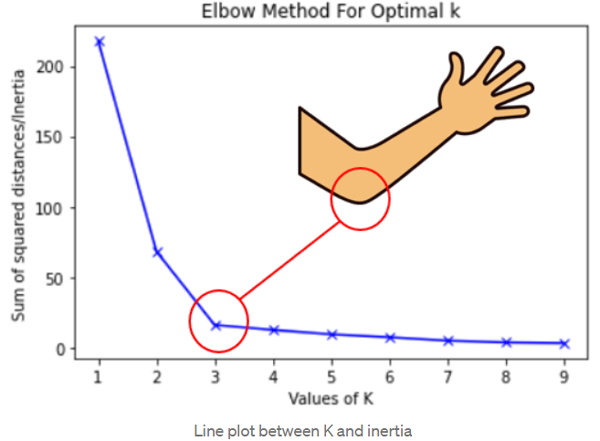
The optimal k value is the k value where increasing it any further would have dramatically less of an impact as increasing it before

Notes

Notes

Udacity, Intro to TensorFlow for Deep Learning

Image Classification with NMIST

CNN with color images

Transfer Learning

Time Series Forecasting

Recurrent Neural Networks (RNN)

Stateful RNN

LSTM Cell (Long Short-Term Memory Cell)

Return of CNNs

Natural Language Processing (NLP)

Text Generation

N-grams

Generative Adversarial Networks (GANs)

Gradient-Based Learning

Neural Net from Scratch

Unsupervised Learning

Principle Component Analysis (PCA)

K-means Algorithm

results matching ""

No results matching ""