Gradient-Based Learning
Here we will explore that magical process by which machines learn. First, we need a metric by which we can measure the performance of the model. This is like defining what we want the model to be good at. For example, if you were to command someone to “get good at drawing,” they would likely ask you what exactly it means to be “good at drawing.” Similarly, this metric defines what the model needs to “get good at,” and it is called the loss function.
Let us define a simple model with one learnable parameter, $A$. A learnable parameter is a number, usually either a weight or a bias, that is adjusted during training. In this case, let us ignore how exactly $A$ is relevant to the output of the model and instead create an arbitrary loss, or objective function: \(L(A)\)
We want to minimize this function; you can think of it as an error function. So how do we minimize this function by changing the parameters of the model, in this case $A$? The answer is calculus! If we compute the derivative of $L(A)$ with respect to $A$, $L’(A)$, then we know how changing $A$ will change the loss function, which we can use to update $A$.
Let’s say that the derivative is greater than 0. Since we are trying to minimize $L(A)$, this means we want to decrease $A$. This logic applies in the opposite sign; in other words, we want to update $A$ in the opposite sign of the derivative. Finally, we want to incorporate some sort of “step size,” since sometimes derivatives can be very large or very small. This step size, call it $\delta$, will simply be multiplied by the derivative when updating $A$, and can change. Thus, we arrive at this simple formula to update $A$:
\[A_{new} = A_{old}-\delta \frac{dL}{dA}\bigg|_{A=A_{old}}\]When we iteratively perform this for a few steps, we essentially descend the gradient, or slope, of the loss function.
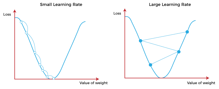
Gradient descent, along with the importance of the step size, or learning rate. In this case a smaller learning rate is optimal to more predictably descend the loss function
This is why this process of iteratively optimizing the model is called gradient descent. Ok, that’s great and all, but how does this scale to a larger model with more learnable parameters? Very simply, we change our loss function to now take in input, $x$, and the parameters, $\theta$:
\[L(x,\theta)\]That’s all, right? Wrong. Now the question becomes: how do we calculate the gradient for each of the parameters to update them, especially in a model with multiple layers? For that, we need backpropagation.
What is backpropagation?
Backpropagation is the process by which the gradient of the loss is calculated with respect to each of the learnable parameters. In this case, we are talking about backpropagation in the context of fully connected networks, although it can be adapted for any type of network.
 A fully connected network
We also need to understand how the model calculates the output from the input. In a fully connected network, every neuron is connected to all of the neurons of the previous layer—in this way, it is “fully connected.” Each neuron multiplies each of the outputs of the previous layer with its own learnable parameter, called a weight. There is a different weight for each of the outputs from the previous layer. These are then summed together and added to another learnable parameter, the bias. For fast computation, this is modeled with matrices. Let us define $z_i$ as the output of the $i$th neuron, $w_i$ as the set of weights of the $i$th neuron, and $b_i$ as the bias for the $i$th neuron, and $x_1$, $x_2$, and $x_3$ as the three inputs of the layer. Through this process we get:
\[\begin{bmatrix} z_1\\z_2\\z_3\\z_4 \end{bmatrix} = \begin{bmatrix}-&w_1^T&-\\-&w_2^T&-\\-&w_3^T&-\\-&w_4^T&-\end{bmatrix}\begin{bmatrix} x_1\\x_2\\x_3\end{bmatrix}+\begin{bmatrix} b_1\\b_2\\b_3\\b_4\end{bmatrix}\]with each $w_i$ having three weights. Note that the dimensions match up:
\[(4,1) = (4,3)*(3,1)+(4,1)\]With the dimensions of multiplying matrices following $(a,b)*(b,c) = (a,c)$. With the appropriate definitions we can write this as
\[z = Wx +b \tag{1}\]Finally, an activation function is applied element-wise (the function is applied independently to each value) with this vector $z$ to get the actual set of outputs, $a$. Yes, I lied; $z$ is not the actual set of outputs but the set just before it.
\[a = \sigma(z)\]Our model applies this operation to the output of each layer to get $\hat{y}$ from the last layer. Remember that the output of one layer is the input of the next. Finally, let us define the loss very simply as $y-\hat{y}$. Now, after defining these things, we can get to backpropagation. Specifically, the question is: how do we calculate the gradient of the loss with respect to every weight and bias? Here is the answer:
\[\frac{\partial L}{\partial W_j}=\frac{\partial L}{\partial a_j}\frac{\partial a_j}{\partial z_j} \frac{\partial z_j}{\partial W_j} \tag{2}\]Where the subscript $j$ means we are referring to each of the $W$, $a$, and $z$ of the $j$th layer. The fancy symbol $\partial$ means that we are taking the partial derivative, which is like a normal derivative, but you treat everything as a constant (except whatever the derivative is taken with respect to). From this we see that
\[\frac{\partial z_j}{\partial W_j} = x = a_{j-1}\]which follows from $(1)$. Similarly we can extend this to the gradient of the $i$th bias of the $j$th layer, $\frac{\partial L}{\partial b_i}$, noting that
\[\frac{\partial z_j}{\partial b_j} = 1\]How do we extend this to models with many layers? $\frac{\partial L}{\partial a_j}$ in $(2)$ becomes
\[\frac{\partial L}{\partial a_j} = \frac{\partial L}{\partial a_{j+1}}\frac{\partial a_{j+1}}{\partial z_{j+1}}\frac{\partial z_{j+1}}{\partial a_j}\]Which you can then apply to find $\frac{\partial L}{\partial a_j}$ for any $j$, noting that by our definition
\[\frac{\partial L}{\partial a_{last}} = y-\hat{y}\]This is where the name “backpropagation” comes from, since you propagate the error, or loss, backwards layer by layer. And that’s all! Very simple!
So it’s just the chain rule?
Yes.
Some clarifications:
\(\frac{\partial z_{j+1}}{\partial a_j}=W_j\) by $(1)$, noting that for every layer $a$ becomes the input $x$ for the next layer.
$\frac{\partial a}{\partial z}$ is the derivative of the activation function. For the sigmoid activation function, this is given by
\[\sigma'(x) = \sigma(x)(1-\sigma(x))\]which makes its calculation pretty simple. A proof can be found here.
Once the gradient is calculated, the weights and biases are updated like this:
\[W_j = W_j-\delta \frac{\partial L}{\partial W_j}\] \[b_j = b_j-\delta \frac{\partial L}{\partial b_j}\]To see all of this applied, check out my neural network made from scratch!