Neural Network From Scratch
Here I will post results and what I learned from neural network from scratch (only numpy) project, which can be found at this link: https://www.kaggle.com/code/zafirnasim/nnfromscratch
I used my knowledge of gradient-based learning and backpropagation, as well as some example notebooks, to create this network from scratch. This notebook in particular was especially helpful, especially for using pandas.


The three Iris species used in the famous Iris flower dataset
Iris Setosa, Iris Versicolour, Iris Virginica
The code in the notebook is my second version, where I turned everything into functions. The original version had a set architecture of (4,5,3), the same as the original notebook that I used for reference. In this newer version, I can make any model architecture and train it by calling only a few functions, which I think is really cool!
The Functions
def initweights(archt):
    if len(archt)<3:
        raise ValueError("architecture needs atleast 1 hidden layer")
    # input is architecture of model, e.g. (4,5,3), needs at least 3 layers
    # output is model in the form [(w1,b1),(w2,b2)...]

    model = []
    for i in range(1,len(archt)):
        w = 2*np.random.random((archt[i-1],archt[i]))-1
        b = 2*np.random.random((1,archt[i]))-1
        model.append([w,b])
    return model
This function initializes the model. The architecture needs to be at least three layers because otherwise the backpropagation function doesn’t work since it’s a bit janky. It initializes the random values in the range [-1.0, 1.0) (np.random.random returns random floats in the interval [0.0, 1.0)) and with the correct dimensions to support forward and backward propagation.
def forwardmodel(model,act,X):
    out = X
    ret = []
    for i,layer in enumerate(model):
        out = np.dot(out,layer[0])+layer[1]
        out = act(out)
        ret.append(out)
    return ret
This function calculates the output of the model given the input by running a forward pass. It’s really simple since the operations are optimized through linear algebra. As described in the gradient-based learning section, it is simply calculating
\[\text{activation}(Wx+b)\]for every layer. ret[-1], the last output, is the final output of the model.
def backprop(model,fwret,dact,X,Y):
    # input is the model, result of forwardprop, derivative of activation function, and data
    # output is gradient in the same form as the model

    grad = [(0,0) for i in range(len(fwret))]
    dl = (Y-fwret[-1])*dact(fwret[-1]) # assuming loss function = 0.5(Y-Y_hat)^2
    for i in range(len(fwret)-1,0,-1):
        if i!=len(fwret)-1:
            dl = np.dot(dl,model[i+1][0].T)*dact(fwret[i])
        grad[i] = (np.dot(fwret[i-1].T,dl),np.dot(np.ones((1,dl.shape[0])),dl))

    dl = np.dot(dl,model[1][0].T)*dact(fwret[0])
    grad[0] = (np.dot(X.T,dl),np.dot(np.ones((1,dl.shape[0])),dl))
    return grad
This function is the sacred backpropagation function. dl is the derivative of the loss with respect to each loss that is carried through the model backwards. As it is carried through, the derivatives with respect to the weights and biases, calculated as described in the gradient-based learning section, are added to the grad list. Thus, the process of updating them looks a lot better than this code.
def acc(model,act,X,Y):
    return sum(forwardmodel(model,act,X)[-1].argmax(axis=1)==Y.argmax(axis=1))/len(X)
This is the code for calculating the accuracy of the model. I knew I could do it in one line, so I had to. What can I say?
error,accu=[],[]
lr = 0.01 # the learning rate
for epoch in range(1000): # 1000 epochs
    fwret = forwardmodel(model,sigmoid,X)
    grad = backprop(model,fwret,dsigmoid,X,Y)
    for i in range(len(model)):
        model[i][0]+=lr*grad[i][0] # weight
        model[i][1]+=lr*grad[i][1] # bias
    error.append(abs(0.5*np.square(Y-fwret[-1])).mean())
    accu.append(acc(model,sigmoid,X,Y))
Here is the code for the actual learning process. In this code snippet, I’m using the sigmoid activation function, which got the best results in my tests, but I also added the ReLU function to try it out.
Since the gradient output of the backpropagation is in the same format as the model, updating the parameters is very simple. Other than that, the code is pretty self-explanatory. The operator for updating the parameters is += instead of -= because the original calculation of dl already factors in a negation; the derivative of the loss function $0.5(y-\hat{y})^2$ should be $-(y-\hat{y})$ but instead it is calculated as $y-\hat{y}$.
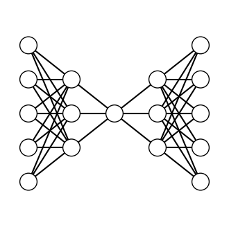
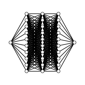
A funky model; (5,3,1,3,5)
Because of these awesome functions, I can make any model with any architecture I choose. Obviously, some are better than others, but most reach at least 95% accuracy by 10,000 epochs on the Iris dataset.
Modelling Functions
My neural network works pretty well on the Iris dataset, but theoretically it should be able to model any function! I tried to model sin(x) and similar functions; here are my results:
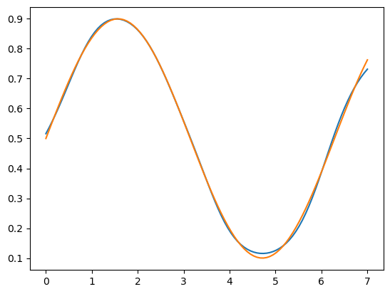
Approximating $0.4\text{sin}(x)+0.5$ in 10000 epochs, mean abs error of 0.0003048
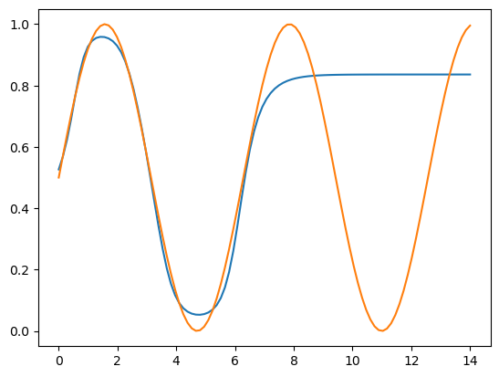
Approximating $0.5\text{sin}(x)+0.5$ from 0 to 14 when it was only trained on 0 to 7; as you can see, it can neither extrapolate well, nor reach values near 1 because of the sigmoid activation function
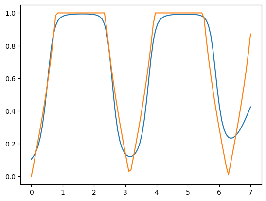
Approximating $\text{min}(\text{abs}(\text{tan}(x)),1)$; not $\text{tan}(x)$ because of the limitations of sigmoid
The model I used for the approximations; (1,10,10,10,1)