Zafir's Blog
Ideas from Gaussian Splatting
Jun 13, 2026Gaussian splatting is a technique used to go from a set of 2D photos of a subject to a realistic 3D representation. The final output is both light enough for real-time rendering and accurate enough for novel view synthesis. It sounds like magic!
| lego | ship |
|---|---|
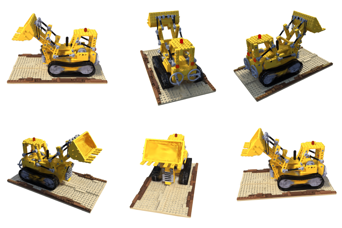 | 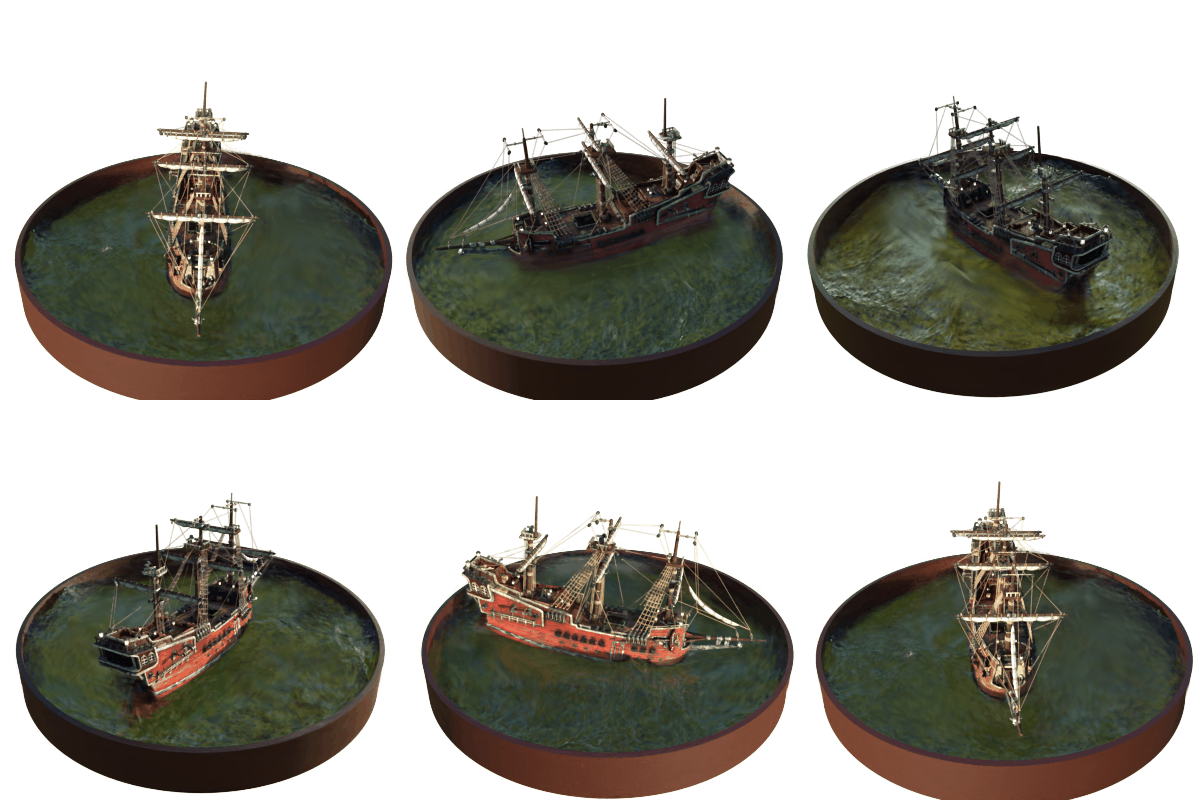 |
To get a feeling for how it works, I decided to implement it (zaforf/torch-splatting). But if you were to read the code alone, you might miss some of the really beautiful ideas.
Efficient, learnable Gaussians
The core idea of Gaussian splatting is representing a 3D model as tons and tons of Gaussians (potentially millions). Each of these Gaussians is parameterized by a mean, which is a 3D point, and a covariance matrix $\Sigma$, which, critically, must be positive semi-definite (PSD).
Review: Why must covariance be PSD?
Intuitively, negative variance for a normal 1D Gaussian makes no sense. This is the higher-dimensional equivalent. Recall that ordinary variance can be defined as $$ \sigma^2 = \frac{1}{n}\sum{(x_i - \bar{x})^2} $$ Similarly, covariance can be defined as $$ \Sigma = \frac{1}{n}\sum{(x_i - \bar{x})(x_i - \bar{x})^{\textsf{T}}} $$ Here $x_i = (x_{i1}, \ldots, x_{id})^{\textsf{T}}$, so the data points are column vectors and each summand is an outer product with dimension $d \times d$. Now consider some vector $y \in \mathbb{R}^d$: $$ \begin{aligned} y^{\textsf{T}}\Sigma y &= y^{\textsf{T}}(\frac{1}{n}\sum{(x_i - \bar{x})(x_i - \bar{x})^{\textsf{T}}})y \\ &= \frac{1}{n}\sum{(y^{\textsf{T}}(x_i - \bar{x}))((x_i - \bar{x})^{\textsf{T}}y)} \\ &= \frac{1}{n}\sum{((x_i - \bar{x})^{\textsf{T}}y)^2} \ge 0 \end{aligned} $$ as $y^{\textsf{T}}(x_i - \bar{x}) = (x_i - \bar{x})^{\textsf{T}}y$. Since this holds for arbitrary $y$, $y^{\textsf{T}}\Sigma y \ge 0$, $\Sigma$ is PSD.This means we cannot naively optimize the 6 degrees of freedom of a $3 \times 3$ symmetric covariance matrix. Instead, we decompose $\Sigma$ as:
- $S$ (scale): a 3D vector $s \in \mathbb{R}^3$ is directly optimized, and to guarantee positive variance we set $S = \text{diag}(\exp(s))$
- $R$ (rotation): a quaternion $q \in \mathbb{R}^4$ is directly optimized, normalized to unit length after every update
Then, $\Sigma = R \cdot S \cdot S^\textsf{T} \cdot R^\textsf{T} = R \cdot S^2 \cdot R^\textsf{T}$ is PSD because it can be written as $(RS)(RS)^\textsf{T}$, and by the spectral theorem it has the right form to represent general covariance shapes.
Why quaternions?
If we directly optimized a $3 \times 3$ rotation matrix $R$ we would again be subject to annoying constraints:
- $R^\textsf{T}R = I$ (orthogonal with unit-length columns)
- $\det(R) = +1$ (as opposed to $-1$, a reflection)
Another straightforward approach is Euler angles, but they suffer from a problem called gimbal lock, where one axis of rotation can be lost.
Quaternions resolve these issues. With four numbers, they are written as an extension of the complex numbers ($q = w + xi + yj + zk$), following similar rules:
\[i^2 = j^2 = k^2 = ijk = -1\]This is enough to derive the other identities, for example:
\[\begin{aligned} i j k &= -1 \\ i j k^2 &= -k \\ -i j &= -k \\ i j &= k \end{aligned}\]These four numbers are directly optimized, and with the normalization constraint, $\lVert q \rVert^2 = w^2 + x^2 + y^2 + z^2 = 1$, this leaves 3 degrees of freedom. How can we rotate using some $q$? If we embed the 3D vector we want to rotate $v$ into 4D as a pure quaternion ($w = 0$), then we can define $q$’s rotation as
\[v' = qvq^\ast\]where $q^\ast$ is the conjugate of $q$, negating the sign of all imaginary terms. This is similar to how unit-magnitude complex numbers rotate the plane $\text{span}(1,i)$. If we write $q = \cos \theta + u \sin \theta$, where $u = xi + yj + zk$, then $q$ behaves like a complex number in the plane $\text{span}(1,u)$. But $qv$ alone is really a 4D rotation of quaternion space; it can introduce a real component when applied to a pure quaternion $v$. The sandwich product $qvq^\ast$ cancels that out and lands us back in the pure quaternions, giving an ordinary 3D rotation. To get a better explanation, I recommend looking into it yourself (and explaining it to me 😅).